Convergence to Planewaves for Solutions to Schrödinger's equation

The main goal of this post is to study the following problem: \begin{equation} i \partial_t \phi(t,x) + \partial^2_{xx}\phi(t,x) = 0 \label{maineq} \end{equation} where the unknown function $\phi: \mathbb{R}\times\mathbb{R}\to \mathbb{C}$, subject to the initial condition \begin{equation} \phi(0,x) = H(x) e^{i k x} \label{initdata} \end{equation} where $H(x)$ is the Heaviside function that vanishes on the negative real line and equals 1 on the positive real line.

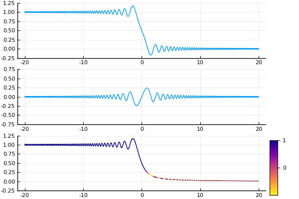
Equation $\eqref{maineq}$ is the free Schrödinger equation on the real line. When the initial data $\phi(0,x)$ is an $L^2$ function, the solution represents the time evolution of (the square root of) a probability distribution of the location of a quantum particle moving on the real line. In our setting, the Heaviside function means that the initial data has actually infinite $L^2$ norm, and so cannot be so easily understood. Nevertheless, we can get a feeling for what the initial data describes, if we remember that the initial data $e^{ikx}$ leads to the monochromatic plane-wave solution \[ \phi(t,x) = e^{-i k^2 t + i k x} \] which travels to the right with velocity (momentum) $k$.

So morally speaking, one may think of the initial data $\eqref{initdata}$ as describing the right-half-line uniformly saturated by particles of fixed momentum $k$. Such an intuition would suggest that the entire solution will propagate to the right with velocity $k$. From the quantum mechanical point of view, of course, such a prescription is impossible: Heisenberg's uncertainty principle precludes us from being able to locate precisely particles with fixed momenta, so in reality we must expect some degree of uncertainty to the actual momenta of our particles. So we may expect that in addition to the bulk motion where the solution propagate with velocity $k$, there will be some blurring of the interface due to the uncertainties of the particle momenta.

This post will examine this problem from a mathematical point of view.

Solving the free Schrödinger equation

The equation $\eqref{maineq}$ has constant coefficients, and formally we can treat it by taking its spatial Fourier transform. Denoting by \[ \hat{\phi}(t,k) = \frac{1}{\sqrt{2\pi}} \int_{\mathbb{R}} \phi(t,x) e^{-ikx} ~\mathrm{d}x \] and ignoring issues of convergence of the actual integral, we see that we can rewrite Schr&omul;dinger's equation as \begin{equation} i \partial_t \hat{\phi}(t,k) - k^2 \hat{\phi}(t,k) = 0 \end{equation} which for fixed $k$ is a simple ordinary differential equation in the time variable $t$, whose solution is given by \begin{equation}\label{fouriersoln} \hat{\phi}(t,k) = e^{-itk^2} \hat{\phi}(0,k). \end{equation} Again ignoring any possible convergence issues, we can take the inverse Fourier transform and obtain the representation formula \[ \phi(t,x) = \frac{1}{\sqrt{2\pi}} \int_{\mathbb{R}} e^{-itk^2} \hat{\phi}(0,k) e^{ikx} ~\mathrm{d}k. \] We can rewrite the mapping from $\phi(0,x)$ to $\phi(t,x)$ through a series of operators: \begin{equation}\label{operatorformula} \phi(t,x) = U_t \phi(0,x) := \mathcal{F}^{-1} M_t \mathcal{F} \phi(0,x) \end{equation} where $\mathcal{F}$ is the Fourier transform, and $M_t$ is the multiplication operator multiplying a function $f(k)$ by $e^{-itk^2}$.

Classical case of Schwartz initial data

To clean-up the discussion above, we have to examine when the expression $\eqref{operatorformula}$ makes sense. The simplest case is when the initial data $\phi(0,x) \in \mathcal{S}$ is a Schwartz function¹. It is well-known that the Fourier transform $\mathcal{F}$ is a linear isomorphism (of topological vector spaces) of the Schwartz space $\mathcal{S}$ to itself². The function $k \mapsto e^{-itk^2}$ is a smooth function with the property that all its derivatives have at most polynomial growth. (Such functions are sometimes called slowly growing smooth functions.) One easily sees that multiplication by such functions gives a bounded mapping of $\mathcal{S}$ to itself³. This implies that the solution operator $U_t$ is a bounded linear map from $\mathcal{S}$ to itself.

Now, were $M_t$ a multiplication by a Schwartz function, then the basic properties of the Fourier transform (which interchanges multiplication and convolution) would imply that there exists some $K_t\in \mathcal{S}$ such that $U_t f = K_t * f$ for every $f\in \mathcal{S}$. While the function $e^{-itk^2}$ is not Schwartz, a similar formula also holds when we regard it as a tempered distribution. A standard calculation shows that the convolution formula actually holds with \begin{equation} \label{schkernel} K_t(x) = \frac{e^{-i \cdot \mathrm{sgn}(t)\cdot \frac{\pi}{4}}}{\sqrt{4\pi |t|}} e^{i \frac{x^2}{4t}} . \end{equation}

Distributional initial data

Since $U_t: \mathcal{S}\to\mathcal{S}$ is bounded (and hence continuous, since $\mathcal{S}$ is Montel⁴), its transpose (which we will denote by $U_t'$) is a bounded linear map from $\mathcal{S}'$, the space of tempered distributions to itself⁵. This implies that the initial value problem for $\eqref{maineq}$ can be solved with $\phi(0,x) = f(x) \in \mathcal{S}'$ with the solution $\phi(t,x) = (U'_{-t})f$.

This in particular implies that the initial data problem for $\eqref{maineq}$ with data $\eqref{initdata}$ is wellposed with solutions that are tempered distributions spatially.

When acting on $f\in \mathcal{S}$, a direct computation shows that $U_t' = U_{-t}$ (taking advantage of the time reversibility of the equation). A natural question then is: does a formula like $\eqref{schkernel}$ hold for data that is a tempered distribution? In our context, one may ask: since that are initial data $\eqref{initdata}$ is in fact piecewise smooth and bounded, can the solution be represented as a function (and not just a distribution), and if so, is there a good representation formula that allows us to get pointwise estimates on the solution?

That the answer is in the positive is perhaps not surprising. Before addressing the full answer, let's consider one property of the kernel $K_t$. Notice that for a fixed $t \neq 0$, $K_t$ is a smooth function of $x$ with constant absolute value. So it is far from being absolutely integrable. However⁶:

The same technique can be used to prove the following.

(I leave the proof to the reader. The key is in integrating $\int_1^b f(x) K_t(x) ~\mathrm{d}x$ by parts twice and arguing similarly as above.)

The same method of proof also gives rise to the following statement⁷:

Corollary 3 does not directly apply to our initial data, which is not differentiable at the origin. But we will channel its spirit in a later section.

Dispersive decay for Schwartz data

Returning for the moment to Schwartz initial data. The idea behind dispersive PDEs is that the rapid decay of the initial data implies that the data describes a spatially concentrated collection of wave packets. By Heisenberg's uncertainty principle the momenta of the wave packets cannot be too concentrated. And the wave packets will travel at different velocities and thereby spread out over time, leading to the local amplitude to decay.

This statement is captured by the (trivial) uniform decay estimate that states \begin{equation}\label{dispest} |K_t * f(x)| \leq \frac{1}{\sqrt{4\pi |t|}} | f|_{L^1(\mathbb{R})}. \end{equation} One way to understand this inequality is the statement that suitably localized initial data (remembering that $L^1$ functions tend to be more "concentrated" than $L^2$ functions) converges uniformly to the steady-state solution that is uniformly 0.

In our setting, however our initial data $\eqref{initdata}$ has infinite energy, and therefore we cannot reasonably expect uniform convergence of the solution to the 0 solution.

Asymptotics for half-line initial data

Denote by $H_k$ the function \[ H_k(x) = H(x) e^{ikx}. \] I claim that it suffices to study the convolution $K_t * H_k $. Using that outside a neighborhood of the origin $H_k$ is smooth with uniformly bounded derivatives, the integration by parts argument used to prove Theorem 2 also suffices to guarantee that $K_t * H_k$ is well-defined as a function.

If, in the definition of $H_k$, instead of the Heaviside function we use a smooth step function, then Corollary 3 applies and the smoothed version of $K_t * H_k$ is the solution to $\eqref{maineq}$. By approximating $H_k$ by mollified versions, the mollified versions converge to $H_k$ in the sense of distributions, and therefore the corresponding solutions (using that the solution operator is continuous on $\mathcal{S}'$) also must converge, in the sense of distributions to the actual solution.

Lastly, using $\eqref{dispest}$ we see that the solutions corresponding to mollified initial data must converge to $K_t * H_k$ uniformly when $t \neq 0$, and hence we have that $K_t * H_k$ is continuous for $t \neq 0$ and must also be the function that represents the distribution that solves $\eqref{maineq}$ with $H_k$ initial data.

It turns out that $K_t * H_k$ has a pretty simple formula. Here we give the "physicist-style" computations; the computations can be rigorously justified by testing against an abstract test function in $\mathcal{S}$, we omit the details.

To start, observe that for $t > 0$ \[ K_t * H_k(x) = \frac{e^{- i \pi / 4}}{2 \sqrt{\pi t}} \int_0^\infty e^{i (x-y)^2 / (4t)} e^{i k y} ~\mathrm{d}y. \] We can expand \[
\frac{(x-y)^2}{4t} + ky = \left( \frac{x}{2\sqrt{t}} - \frac{y}{2\sqrt{t}} - \sqrt{t} k\right)^2 + kx - t k^2 \] to rewrite \[ K_t * H_k(x) = \frac{e^{- i\pi/4}}{2 \sqrt{\pi t}} e^{ik(x - kt)} \int_0^\infty e^{i ( x/\sqrt{4t} - y / \sqrt{4t} - \sqrt{t}k )^2} ~\mathrm{d}y. \] Next perform the change of variables $z = y / \sqrt{4t}$ we get \[ K_t * H_k(x) = \frac{e^{- i\pi/4}}{\sqrt{\pi}} e^{ik(x - kt)} \int_0^\infty e^{i ( x/\sqrt{4t} - z - \sqrt{t}k )^2} ~\mathrm{d}z \] and a further change of variables gives \begin{equation}\label{explicitsoln} K_t * H_k(x) = \frac{e^{- i\pi/4}}{\sqrt{\pi}} e^{ik(x - kt)} \int_{\sqrt{t}k - x / \sqrt{4t}}^\infty e^{i z^2} ~\mathrm{d}z. \end{equation} The integral can be written in terms of the (complex) complementary error function: \[ \mathsf{erfc}\bigl( \frac{1 - i}{\sqrt{2}} \cdot w \bigr) := \frac{2e^{-i\pi/4}}{\sqrt{\pi}} \int_w^\infty e^{i z^2} ~\mathrm{d}z. \]

Using the formulation in terms of the complementary error function $\mathsf{erfc}$, we can easily visualize the behavior of the solutions numerically: the solution $\eqref{explicitsoln}$ states that, up to a phase modulation by the traveling wave $e^{ik(x-kt)}$, the amplitude of the solution is given by the $\mathsf{erfc}$ function translated by $2tk$ and rescaled by $(4t)^{-1/2}$.

What's interesting to note, is that the "wavefront" is traveling at speed $2k$ (note that the planewave it starts with has momentum $k$). This can be seen in the bottom two graphs in the figure: at time $t = 10$ the wavefront exits the field of view of $x\in [-40,40]$, starting out from $x = 0$. The two figures represent $k = \pm 2$ respectively, and the wavefront is traveling at speed 4. What we see here, of course, is the difference between the phase velocity and group velocity. For Schrödinger equation, the dispersion relation is $\omega = k^2$. So the phase velocity (the speed at which the crests of the monochromatic plane-wave propagates) is $\omega / k = k$, while the group velocity (the speed at which the envelope of a wave packet propagates) is $\partial\omega / \partial k = 2k$. This can also be seen pretty clearly in the bottom plot. The "waviness" of the graph shows the amplitude modulation and captures the envelope of the wave group, while the color of the graph shows the phase modulation. Relative to the crests and troughs of the amplitude modulation, the colored segments (representing points of constant phase) seems to be moving to the right, when in fact both the amplitude and phase modulations are traveling to the left. (Indicating that the amplitude modulation is traveling faster than the phase modulation.)

The formula $\eqref{explicitsoln}$ also immediately allows us to read off the asymptotic behaviors.

• When $k = 0$ the waveform does not move, and merely dilates. This means that we can expect the solution to converge (pointwise in amplitude) to $|\frac12\mathsf{erfc}(0)| = \frac12$.
• When $k > 0$, the waveform travels to the right. Notice that the waveform travels at speed $\propto |t|$ while dilates at rate $\propto t^{-1/2}$, so the translation beats the dilation. This means that we can expect the solution to converge (pointwise in amplitude) to $0$.
• When $k < 0$, the waveform travels to the left. This means similarly that we can expect the solution to converge (pointwise in amplitude) to $1$.

These are borne out in the figure below.

It is worth noting that the convergence can only ever be pointwise: uniform convergence is not possible since in all cases, by $\eqref{explicitsoln}$ we see that for all times $t$ \[ \inf |K_t * H_k| = 0 < \frac12 < 1 \leq \sup |K_t * H_k| .\]

Another interesting thing to note is the phase properties. In two cases where $k = 0$ or $k > 0$, the figures above suggest that on compact intervals the solution approach having constant phase in addition to having constant amplitude. Physically this is reasonable as the "particles" that are left over in these cases should be the ones that are not moving, and hence should have zero frequency. In the case where $k < 0$ we should converge toward a stream of particles moving with momentum $k$ coming in from $+\infty$, and therefore we do expect convergence toward a monochromatic plane-wave.

Now let us examine the asymptotic properties at fixed $x$ of $K_t * H_k(x)$.

$k = 0$

When $k = 0$, we have by $\eqref{explicitsoln}$ that \[ K_t * H_0(x) = \frac12 \mathsf{erfc}\bigl( -\frac{(1 - i)x}{\sqrt{8t}} \bigr) .\] As already discussed above the limit approaches 1/2. Since the error function $\mathsf{erf}$ is an entire function, it is equal to its Maclaurin series, and hence we can read off exactly \[ K_t * H_0(x) = \frac12 + \frac1\pi \left( e^{-i\pi/4} \frac{x}{2\sqrt{t}} - e^{-i 3\pi/4} \frac{x^3}{24 t^{3/2}} + e^{-i 5\pi/4} \frac{x^5}{320 t^{5/2}} + \cdots \right).\] And hence on any compact subset of $\mathbb{R}$, $K_t * H_0$ converges uniformly, with rate $t^{-1/2}$, to 1/2. (Note that we have shown the solution converges to a constant, and therefore captured both the amplitude and phase convergence observed in the figures.)

$k > 0$ (particles move to the right)

When $k > 0$ we can bound the solution using oscillatory integral techniques. Our explicit solution yields \[ K_t * H_k(x) = e^{ik(x-kt)} \cdot \frac{e^{-i\pi/4}}{\sqrt{\pi}} \int_{\sqrt{t} k - x / \sqrt{4t}}^\infty e^{iz^2} ~\mathrm{d}z. \] That $\int e^{iz^2} ~\mathrm{d}z$ converges implies that as $t\to+\infty$ this value will converge to 0. To see the rate of convergence, we can assume, without loss of generality, that $2kt > x$, so that on the interval $(\sqrt{t}k - x/\sqrt{4t}, \infty)$ the function $z^2$ has no critical points. By Van der Corput Lemma, we must have⁸ \[ \left| \int_{\sqrt{t} k - x / \sqrt{4t}}^\infty e^{iz^2} ~\mathrm{d}z \right| \leq \frac{3}{2 \sqrt{t} k - x / \sqrt{t}} .\] This means that we also have $t^{-1/2}$ uniform convergence on compact subsets to $0$.

$k < 0$ (particles move to the left)

When $k < 0$, we can similarly bound the solution. The explicit solution yields \[ K_t * H_k(x) = e^{ik(x-kt)} \cdot \left( 1 - \frac{e^{-i\pi/4}}{\sqrt{\pi}} \int_{-\infty}^{\sqrt{t} k - x / \sqrt{4t}} e^{iz^2} ~\mathrm{d}z \right). \] The same Van der Corput Lemma argument gives now that we have uniform convergence on compact subsets, at rate $t^{-1/2}$, to the traveling monochromatic plane wave $e^{ik(x-kt)}$.

The big picture

Combining the three regimes together with Remark 4, we can conclude the following:

With $H_k$ initial data, an observer moving at velocity $v < 2k$ will see, in his neighborhood, the solution converge uniformly to 0. An observer moving at velocity $v > 2k$ will see, in his neighborhood, the solution converge uniformly to the monochromatic plane-wave with momentum $k$. And finally, an observer moving at exactly velocity $v = 2k$ will see, in his neighborhood, the solution converge uniformly to to the constant solution $1/2$. In all three cases the convergence happens with rate $t^{-1/2}$. In the first two cases the constant depends on $v - 2k$.