Simulating Closed Cosmic Strings

One of my current research interests is in the geometry of constant-mean-curvature time-like submanifolds of Minkowski space. A special case of this is the study of cosmic strings under the Nambu-Goto action. Mathematically the classical (as opposed to quantum) behavior of such strings are quite well understood, by combining the works of theoretical physicists since the 80s (especially those of Jens Hoppe and collaborators) together with recent mathematical developments (such as the work of Nguyen and Tian and that of Jerrard, Novaga, and Orlandi). To get a better handle on what is going on with these results, and especially to provide some visual aids, I've tried to produce some simulations of the dynamics of closed cosmic strings. (This was also an opportunity for me to practice code-writing in Julia and learn a bit about the best practices for performance and optimization in that language.)

The code

After some false starts, here are some reasonably stable code.

MeanCurvature3.jl:

function MC_corr3!(position::Array{Float64,2}, prev_vel::Array{Float64,2}, next_vel::Array{Float64,2}, result::Array{Float64,2}, dt::Float64)
  # We will assume that data is stored in the format point(coord,number), so as a 3x1000 array or something. 
  num_points = size(position,2)
  num_dims = size(position,1)

  curr_vel = zeros(num_dims)
  curr_vs = zeros(num_dims)
  curr_ps = zeros(num_dims)
  curr_pss = zeros(num_dims)

  pred_vel = zeros(num_dims)
  agreement = true

  for col = 1:num_points  #Outer loop is column
    if col == 1
      prev_col = num_points
      next_col = 2
    elseif col == num_points
      prev_col = num_points - 1
      next_col = 1
    else
      prev_col = col -1
      next_col = col + 1
    end

    for row = 1:num_dims
      curr_vel[row] = (next_vel[row,col] + prev_vel[row,col])/2
      curr_vs[row] = (next_vel[row,next_col] + prev_vel[row,next_col] - next_vel[row,prev_col] - prev_vel[row,prev_col])/4
      curr_ps[row] = (position[row,next_col] - position[row,prev_col])/2
      curr_pss[row] = position[row,next_col] + position[row,prev_col] - 2*position[row,col]
    end

    beta = (1 + dot(curr_vel,curr_vel))^(1/2)
    sigma = dot(curr_ps,curr_ps)
    psvs = dot(curr_ps,curr_vs)
    bvvs = dot(curr_vs,curr_vel) / (beta^2)
    pssps = dot(curr_pss,curr_ps)

    for row in 1:num_dims
      result[row,col] = curr_pss[row] / (sigma * beta) - curr_ps[row] * pssps / (sigma^2 * beta) - curr_vel[row] * psvs / (sigma * beta) - curr_ps[row] * bvvs / (sigma * beta)
      pred_vel[row] = prev_vel[row,col] + dt * result[row,col]
    end

    agreement = agreement && isapprox(next_vel[:,col], pred_vel, rtol=sqrt(eps(Float64)))
  end

  return agreement
end


function find_next_vel!(position::Array{Float64,2}, prev_vel::Array{Float64,2}, next_vel::Array{Float64,2}, dt::Float64; max_tries::Int64=50)
  tries = 1
  result = zeros(next_vel)
  agreement = MC_corr3!(position,prev_vel,next_vel,result,dt)
  for j in 1:size(next_vel,2), i in 1:size(next_vel,1)
    next_vel[i,j] = prev_vel[i,j] + result[i,j]*dt
  end
  while !agreement && tries < max_tries
    agreement = MC_corr3!(position,prev_vel,next_vel,result,dt)
    for j in 1:size(next_vel,2), i in 1:size(next_vel,1)
      next_vel[i,j] = prev_vel[i,j] + result[i,j]*dt
    end
    tries +=1
  end
  return tries, agreement
end

This first file does the heavy lifting of solving the evolution equation. The scheme is a semi-implicit finite difference scheme. The function MC_Corr3 takes as input the current position, the previous velocity, and the next velocity, and computes the correct current acceleration. The function find_next_vel iterates MC_Corr3 until the computed acceleration agrees (up to numerical errors) with the input previous and next velocities.

Or, in notations:
MC_Corr3: ( x[t], v[t-1], v[t+1] ) --> Delta-v[t]
and find_next_vel iterates MC_Corr3 until
Delta-v[t] == (v[t+1] - v[t-1]) / 2

The code in this file is also where the performance matters the most, and I spent quite some time experimenting with different algorithms to find one with most reasonable speed.

InitialData3.jl:

function make_ellipse(a::Float64,b::Float64, n::Int64, extra_dims::Int64=1)  # a,b are relative lengths of x and y axes
  s = linspace(0,2π * (n-1)/n, n)
  if extra_dims == 0
    return vcat(transpose(a*cos(s)), transpose(b*sin(s)))
  elseif extra_dims > 0
    return vcat(transpose(a*cos(s)), transpose(b*sin(s)), zeros(extra_dims,n))
  else
    error("extra_dims must be non-negative")
  end
end

function perturb_data!(data::Array{Float64,2}, coeff::Vector{Float64}, num_modes::Int64) 
  # num_modes is the number of modes
  # coeff are the relative sizes of the perturbations

  numpts = size(data,2)

  for j in 2:num_modes
    rcoeff = rand(length(coeff),2)

    for pt in 1:numpts
      theta = 2j * π * pt / numpts
      for d in 1:length(coeff)
        data[d,pt] += ( (rcoeff[d,1] - 0.5) *  cos(theta) + (rcoeff[d,2] - 0.5) * sin(theta)) * coeff[d] / j^2
      end
    end
  end

  nothing
end

This file just sets up the initial data. Note that in principle the number of ambient spatial dimensions is arbitrary.

GraphCode3.jl:

using Plots

pyplot(size=(1920,1080), reuse=true)

function plot_data2D(filename_prefix::ASCIIString, filename_offset::Int64, titlestring::ASCIIString, data::Array{Float64,2}, additional_data...)
  x_max = 1.5
  y_max = 1.5
  plot(transpose(data)[:,1], transpose(data)[:,2] , xlims=(-x_max,x_max), ylims=(-y_max,y_max), title=titlestring)
  
  if length(additional_data) > 0
    for i in 1:length(additional_data)
      plot!(transpose(additional_data[i][1,:]), transpose(additional_data[i][2,:]))
    end
  end
  
  png(filename_prefix*dec(filename_offset,5)*".png")
  nothing
end

function plot_data3D(filename_prefix::ASCIIString, filename_offset::Int64, titlestring::ASCIIString, data::Array{Float64,2}, additional_data...)
  x_max = 1.5
  y_max = 1.5
  z_max = 0.9
  tdata = transpose(data)
  plot(tdata[:,1], tdata[:,2],tdata[:,3], xlims=(-x_max,x_max), ylims=(-y_max,y_max),zlims=(-z_max,z_max), title=titlestring)

  if length(additional_data) > 0
    for i in 1:length(additional_data)
      tdata = transpose(additional_data[i])
      plot!(tdata[:,1], tdata[:,2], tdata[:,3]) 
    end
  end

  png(filename_prefix*dec(filename_offset,5)*".png")
  nothing
end

This file provides some wrapper commands for generating the plots.

NonNewton3.jl:

include("InitialData3.jl")
include("MeanCurvature3.jl")
include("GraphCode3.jl")

num_pts = 3000
default_timestep = 0.01 / num_pts
max_time = 3
plot_every_ts = 1500

my_data = make_ellipse(1.0,1.0,num_pts,0)
perturb_data!(my_data, [1.0,1.0], 15)
this_vel = zeros(my_data)
next_vel = zeros(my_data)

for t = 0:floor(Int64,max_time / default_timestep)
  num_tries, agreement = find_next_vel!(my_data, this_vel,next_vel,default_timestep)

  if !agreement
    warn("Time $(t*default_timestep): failed to converge when finding next_vel.")
    warn("Dumping information:")
    max_beta = 1.0
    max_col = 1
    for col in 1:size(my_data,2)
      beta = (1 + dot(next_vel[:,col], next_vel[:,col]))^(1/2)
      if beta > max_beta
        max_beta = beta
	max_col = col
      end
    end
    warn("   Beta attains maximum at position $max_col")
    warn("   Beta = $max_beta")
    warn("   Position = ", my_data[:,max_col])
    prevcol = max_col - 1
    nextcol = max_col + 1
    if max_col == 1
      prevcol = size(my_data,2)
    elseif max_col == size(my_data,2)
      nextcol = 1
    end
    warn("   Deltas")
    warn("    Left:  ", my_data[:,max_col] - my_data[:,prevcol])
    warn("    Right:  ", my_data[:,nextcol] - my_data[:,max_col])
    warn("   Previous velocity: ", this_vel[:,max_col])
    warn("   Putative next velocity: ", next_vel[:,max_col])
    warn("Quitting...")
    break
  end

  for col in 1:size(my_data,2)
    beta = (1 + dot(next_vel[:,col], next_vel[:,col]))^(1/2)
    for row in 1:size(my_data,1)
      my_data[row,col] += next_vel[row,col] * default_timestep / beta
      this_vel[row,col] = next_vel[row,col]
    end

    if beta > 1e7
      warn("time: ", t * default_timestep)
      warn("Almost null... beta = ", beta)
      warn("current position = ", my_data[:,col])
      warn("current Deltas")
      prevcol = col - 1
      nextcol = col + 1
      if col == 1
        prevcol = size(my_data,2)
      elseif col == size(my_data,2)
        nextcol = 1
      end
      warn(" Left: ", my_data[:,col] - my_data[:,prevcol])
      warn(" Right: ", my_data[:,nextcol] - my_data[:,col])
    end
  end

  if t % plot_every_ts ==0
    plot_data2D("3Dtest", div(t,plot_every_ts), @sprintf("elapsed: %0.4f",t*default_timestep), my_data, make_ellipse(cos(t*default_timestep), cos(t*default_timestep),100,0))
    info("Frame $(t/plot_every_ts):  used $num_tries tries.")
  end
end

And finally the main file. Mostly it just ties the other files together to produce the plots using the simulation code; there are some diagnostics included for me to keep an eye on the output.

The results

First thing to do is to run a sanity check against explicit solutions. In rotational symmetry, the solution to the cosmic string equations can be found analytically. As you can see below the simulation closely replicates the explicit solution in this case.

The video ends when the simulation stopped. The simulation stopped because a singularity has formed; in this video the singularity can be seen as the collapse of the string to a single point.

Next we can play around with a more complicated initial configuration.

In this video the blue curve is the closed cosmic string, which starts out as a random perturbation of the circle with zero initial speed. The string contracts with acceleration determined by the Nambu-Goto action. The simulation ends when a singularity has formed. It is perhaps a bit hard to see directly where the singularity happened. The diagnostic messages, however, help in this regard. From it we know that the onset of singularity can be seen in the final frame:

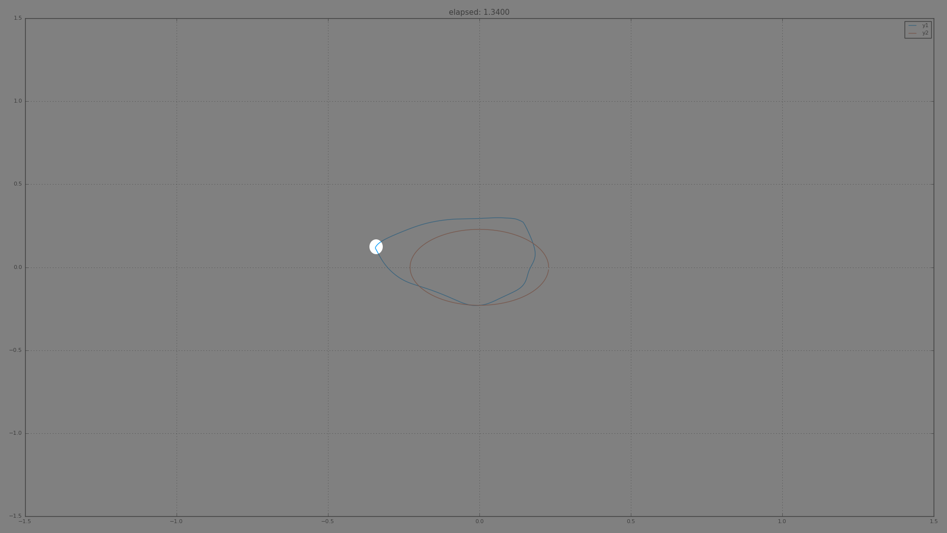
The highlighted region is getting quite pointy. In fact, that is accompanied with the "corner" picking up infinite acceleration (in other words, experiencing an infinite force). The mathematical singularity corresponds to something unreasonable happening in the physics.

To make it easier to see the "speed" at which the curve is moving, the following videos show the string along with its "trail". This first one again shows how a singularity can happen as the curve gets gradually more bent, eventually forming a corner.

This next one does a good job emphasizing the "wave" nature of the motion.

The closed cosmic strings behave like a elastic band. The string, overall, wants to contract to a point. Small undulations along the string however are propagated like traveling waves. Both of these tendencies can be seen quite clearly in the above video. That the numerical solver can solve "past" the singular point is a happy accident; while theoretically the solutions can in fact be analytically continued past the singular points, the renormalization process involved in this continuation is numerically unstable and we shouldn't be able to see it on the computer most of the time.

The next video also emphasizes the wave nature of the motion. In addition to the traveling waves, pay attention to the bottom left of the video. Initially the string is almost straight there. This total lack of curvature is a stationary configuration for the string, and so initially there is absolutely no acceleration of that segment of the string. The curvature from the left and right of that segment slowly intrudes on the quiescent piece until the whole thing starts moving.

The last video for this post is a simulation when the ambient space is 3 dimensional. The motion of the string, as you can see, becomes somewhat more complicated. When the ambient space is 2 dimensional a point either accelerates or decelerates based on the local (signed) curvature of the string. But when the ambient space is 3 dimensional, the curvature is now a vector and this additional degree of freedom introduces complications into the behavior. For example, when the ambient space is 2 dimensional it is known that all closed cosmic strings become singular in finite time. But in 3 dimensions there are many closed cosmic strings that vibrate in place without every becoming singular. The video below is one that does however become singular. In addition to a fading trail to help visualize the speed of the curve, this plot also includes the shadows: projections of the curve onto the three coordinate planes.