In a previous post we discussed a little problem in "almost" Finsler geometry. In this post we will dissect some properties of this geometry a bit more. (And correct a few mistakes in the analyses of the previous post.) It is not exactly necessary to read the previous post first, but skimming it will give you the background of the problem.
The Geometry
We are interested in geodesics, in the sense of length-minimizing curves, on the manifold $(x,y,\theta) \in \mathcal{C} = \mathbb{R}^2 \times \mathbb{S}^1$. Given a curve $\gamma(t) = (x(t), y(t), \theta(t)): [0,1]\to \mathcal{C}$, we denote its lift to the tangent bundle $T\mathcal{C}$ by \begin{equation} T\gamma = (x,y,\theta,\dot{x},\dot{y},\dot{\theta}) \in T\mathcal{C} \cong \mathcal{C}\times \mathbb{R}^3$. \end{equation} The length functional is defined by: \begin{equation} \ell[\gamma] = \int_0^1 F_A(T\gamma(t)) + F_B(T\gamma(t)) ~dt \end{equation} where \begin{gather} F_A(T\gamma) = \sqrt{(\dot{x} - \sin(\theta) \dot{\theta})^2 + (\dot{y} + \cos(\theta)\dot{\theta})^2} \newline F_B(T\gamma) = \sqrt{(\dot{x} + \sin(\theta) \dot{\theta})^2 + (\dot{y} - \cos(\theta)\dot{\theta})^2} \end{gather}
As mentioned in the previous post, this length functional almost defines a Finsler geometry. For a fixed base point $p$, along the fibre $T_p\mathcal{C}$ the function $F_A + F_B$ is
- Positive definite
- Convex
- Positively 1-homogeneous
However, this fails to be a Finsler geometry because the function $F_A + F_B$ is not strongly convex, and, importantly, is not smooth.
To make this extremely evident, below we plot the level surface of $F_A + F_B$ at the point $(x,y,\theta) = (0,0,\pi/2)$. (Notice that the $x$ and $y$ coordinate values are irrelevant since $F_A$ and $F_B$ do not depend on them, but the $\theta$ value does come in play.)
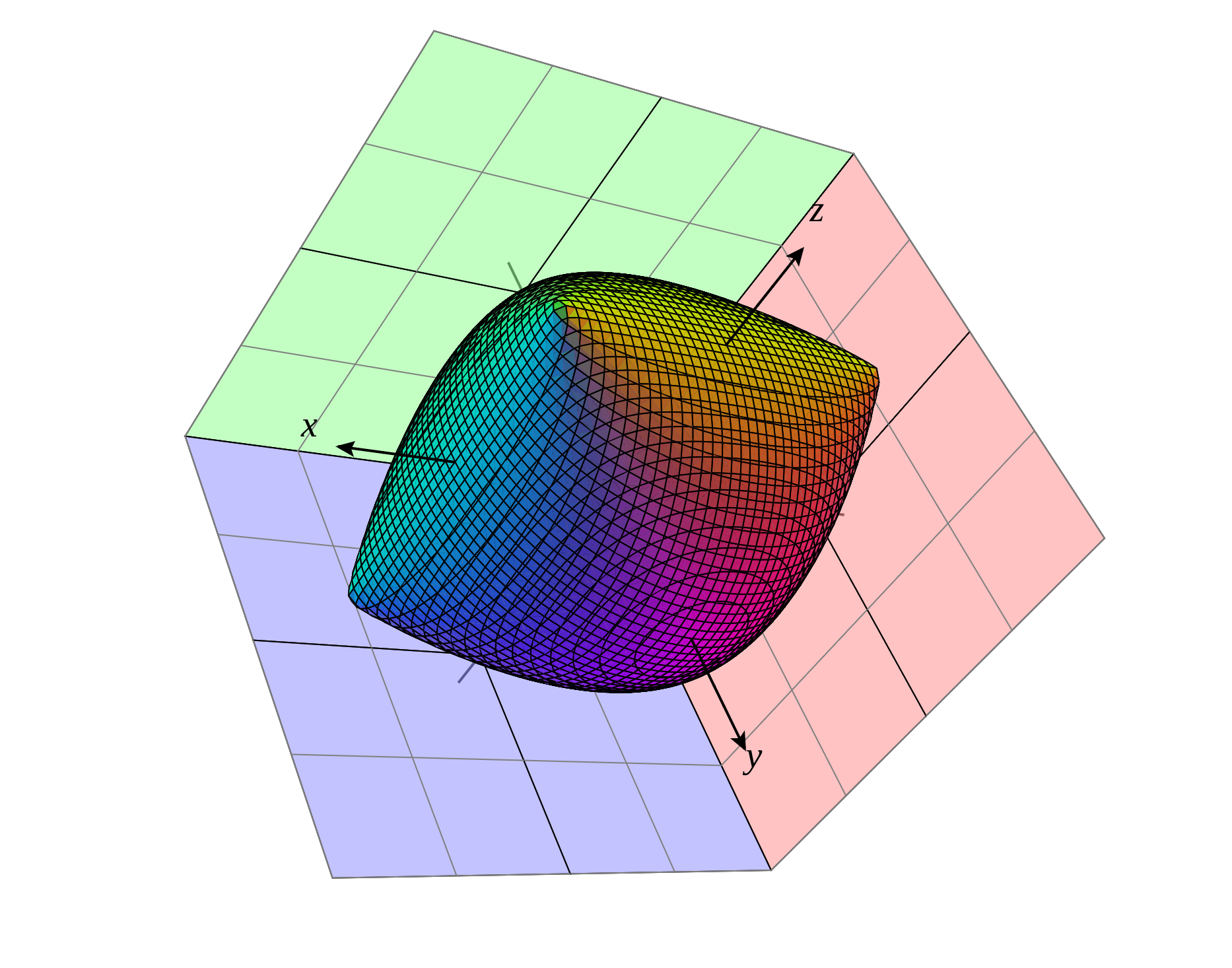
The level set $F_A + F_B = 3$ when $\theta = \pi/2$. The $x$ and $y$ axis represent the values of $\dot{x}$ and $\dot{y}$ respectively, the $z$ axis is the value of $\dot{\theta}$. Figure created using CalcPlot3D and you can access an interactive version of the figure here.
Notice that the level surface is "pillow-shaped".
- The four corners of the pillow are precisely where $F_A + F_B$ are not differentiable.
- The edges of the pillow (where $\dot{y} = 0$) form a square, and this shows that $F_A + F_B$ is not strongly convex.
Analytic implications
Formally computing the Euler-Lagrange equations for minimizing the length functional $\ell$ we find \[\begin{gathered} \frac{d}{dt} \left( \frac{\dot{x}-\sin(\theta) \dot{\theta}}{F_A} + \frac{\dot{x}+ \sin(\theta)\dot{\theta}}{F_B} \right) = 0 \newline \frac{d}{dt} \left( \frac{\dot{y}+\cos(\theta) \dot{\theta}}{F_A} + \frac{\dot{y}- \cos(\theta)\dot{\theta}}{F_B} \right) = 0 \newline \frac{d}{dt} \left( \frac{\dot{\theta}}{F_A} + \frac{\dot{\theta}}{F_B} \right) + \sin(\theta) \frac{d}{dt} \left(\frac{\dot{x}}{F_B} - \frac{\dot{x}}{F_A} \right) + \cos(\theta) \frac{d}{dt} \left(\frac{\dot{y}}{F_A} - \frac{\dot{y}}{F_B} \right) = 0. \end{gathered} \]
There are some caveats on how we should interpret these equations.
Gauge Fixing
First, there is the general problem of reparametrization invariance: if $s:[0,1]\to[0,1]$ is a increasing diffeomorphism, then $\gamma(s(t))$ and $\gamma(t)$ are two distinct parametrizations of the same curve. As functions from $[0,1]\ni t \to \mathcal{C}$, when $s$ is not the identity mapping, the two functions $\gamma\circ s$ and $\gamma$ are distinct. However, the equations of motion above cannot distinguish between $\gamma$ and $\gamma\circ s$; and so the system is in fact underspecified.
This is however a general fact in studying geodesic motion on metric spaces, and is similar to the gauge invariance in studying general relativity. The solution is simple: we gauge fix. A very convenient gauge choice, and this is typically used in Finsler and sub-Riemannian geometries, is the constant speed gauge. This requires that \[ \frac{d}{dt} (F_A + F_B) = 0. \]
In the case of Finsler geometries, with this gauge fixing, we would find that the Euler-Lagrange equations reduce to second order ordinary differential equations for $(x,y,\theta)$, of the form \begin{equation}\label{eq:ODE} \ddot{\gamma} = V(\gamma,\dot{\gamma}) \end{equation} where $V$ is Lipschitz continuous, and hence we can use the usual Picard-Lindelof theorem to guarantee the local wellposedness of the initial value problem.
In particular, in the usual Finsler geometries, we have that starting with a initial $T\gamma(0)$, there is a unique solution to the Euler Lagrange equation.
Singularity
As we discussed in the previous post, one obvious problem with the lack of regularity of $F_A + F_B$ is that it no longer makes sense to study the Euler-Lagrange equations for trajectories that pass through such corner points. (This is precisely the problem where $F_A = 0$ or $F_B = 0$.)
When $F_A = 0$ on an interval (in which case we can assume $F_B > 0$, other wise the trajectory is stationary), necessarily we have that $\dot\theta \neq 0$. In this case we can then parametrize (locally) by $t = \theta$, and hence we have \[ x(\theta) = -\cos\theta, \quad y(\theta) =-\sin\theta. \] Now consider $(\delta_x(\theta), \delta_y(\theta))$ a small perturbation, again parametrized by $\theta$, we find that the length functional of the perturbed curve is \[ \int \sqrt{ \dot{\delta}^2_x + \dot{\delta}^2_y} + \sqrt{ (\dot{\delta}_x - 2 \cos\theta)^2 + (\dot{\delta}_y - 2\sin\theta)^2}. \] This quantity is \[ \geq \int \sqrt{ (2 \cos\theta)^2 + (2\sin\theta)^2} \] by the standard triangle inequality. And hence we see that trajectories where $F_A \equiv 0$ is locally a critical point of the length functional.
Nonuniqueness
However, the fact that our geometry is not Finsler does mean that we no longer have the uniqueness of the initial value problem. This is well-known for ordinary equations of the form \eqref{eq:ODE} where $V$ is merely continuous, but not necessarily Lipschitz.
Observe that for any function $\lambda(\theta)$ taking values strictly between $(-1,1)$, if $x(\theta)$ and $y(\theta)$ solve \[ \dot{x}(\theta) = \lambda(\theta) \sin(\theta), \quad \dot{y}(\theta) = -\lambda(\theta)\cos(\theta), \] we have \[ F_A = 1 - \lambda, \quad F_B = 1 + \lambda \] and so $F_A + F_B = 2$ is constant. These are critical points of the length functional.
Now, given $\lambda_1$ and $\lambda_2$, if it were the case that \[ \lambda_1(a) = \lambda_2(a), \quad \lambda_1(b) = \lambda_2(b) \] and \[ \int_a^b \lambda_1(s) \sin(s) ~ds = \int_a^b \lambda_2(s) \sin(s) ~ ds \] and \[ \int_a^b \lambda_1(s) \cos(s) ~ds = \int_a^b \lambda_2(s) \cos(s) ~ ds \] Then the corresponding trajectories $\gamma_1$ and $\gamma_2$ will have the properties that
- $\ell(\gamma_1) = \ell(\gamma_2)$
- $\gamma_1(a) = \gamma_2(a)$ and $\gamma_1(b) = \gamma_2(b)$
- $\dot{\gamma}_1(a) = \dot{\gamma}_2(a)$ and $\dot{\gamma}_1(b) = \dot{\gamma}_2(b)$.
and we see that the uniqueness of geodesics connecting two points becomes rather severely violated: we have now two distinct trajectories with with the same initial/final location and initial/final velocities, but both are critical points of the length functional.
To see this example panning out: consider the case where $\lambda_0 \equiv 0$, on the interval $[0,\pi]$. This corresponds to flipping the rod over, and has total traversed distance $2\pi$. Let $\lambda_a = a \cdot \sin(4\theta)$. The integrals can be evaluated exactly. For any $a \in (-1,1)\setminus \{0\}$ this gives another geodesic of our problem. They all give total length of $2$. The animation below shows the case $a = 0.8$. The green circle corresponds to the $a = 0$ solution. You can click on the animation and play around with different $a$ values.
So, what makes the previous example work? It turns out that by posing $\dot{x} = \lambda \sin$ and $\dot{y} = -\lambda \cos$, we are restricting the path $\gamma$ so that at every point along $\gamma$, the velocity vector $\dot{\gamma}$ likes along the "pillow's edge", where $F_A + F_B$ is not strictly convex.
In actual Finsler geometry (or in normal geometry if you will), having the strict convexity means that on sufficiently brief intervals, if you replace an actual geodesic with a perturbation, the perturbation will have strictly longer length. But in our problem, the geometry has a portion that looks more like the Taxicab Geometry, which also has the problem with non-unique geodesics. The Example above is a concrete manifestation of this.
Notice now that if a curve $\gamma$ stays away from the pillow's edge, then the usual arguments apply, and in fact we have that the curve is locally length minimizing on short intervals, and therefore we have uniqueness of the corresponding initial value problem.
But what if a curve starts away from the edge, and then moves toward it? Is this possible? The edge corresponds to $(\dot{x}, \dot{y}) \propto (\sin\theta,-\cos\theta)$. Our analysis from the previous post indicates that away from the edge the only local geodesic motion available are those corresponding to linear motions. And if the motion is from parallel motion, then $\dot{\theta} = 0$ and so if we start away from the edge we always stay away from the edge. And hence we are down to looking at the non-parallel linear motions.
Let's start by giving a general formula for the non-parallel linear motions. In this case we have $\dot\theta \neq 0$ and hence we can parametrize by $\theta$. Up to a translation, we can assume the lines traced by $(x + \cos\theta,y+\sin\theta)$ and $(x-\cos\theta,y-\sin\theta)$ intersect at the origin. So there exists an invertible matrix $\begin{pmatrix} a& b \newline c & d\end{pmatrix}$ such that \[ \begin{gathered} a(x + \cos\theta) + b (y + \sin\theta) = 0 \newline c(x - \cos\theta) + b (y-\sin\theta) = 0 \end{gathered} \] Solving this we find that the general solution takes the form \begin{gather} (ad - bc) x(\theta) = - 2bd \sin\theta - (bc+da) \cos\theta \newline (ad - bc) y(\theta) = 2ac \cos\theta + (bc+da) \sin\theta \end{gather}
Below you can see the general solutions with modifiable parameters on Desmos. The purple curve traces out the value of $(x,y)$.
Now, in my previous post, I mentioned that these geodesics terminate after finite time; here it appears that these curves continue indefinitely: what gives? Note that when the end point of the rod approaches the end of the "rail", it must turn around, and will instantaneously have zero speed. This makes it land on one of the four pillow corners. And this gives us our opportunity.
The stationary point happens at $\theta_0$ such that \[ \dot{x}(\theta_0) = \pm \sin(\theta_0), \qquad \dot{y}(\theta_0) = \mp \cos(\theta_0) \] For simplicity, consider the situations where $a = 1 = d$ and $b = 0$; then the stationary points are \[ \theta_0 = \tan^{-1} 0, \tan^{-1} \frac1c. \] At those points, it is possible to match a singular trajectory with $\dot{x} = \pm \sin\theta$ and $\dot{y} = \mp \cos\theta$ to obtain a $C^1$ curve that jumps from the linear-trajectory to a purely rotating one. See the illustration below.
This joining is also itself non-unique: by virtue of Example 1, we can also join to any singular trajectory with $\dot{x} = \pm \lambda(\theta) \sin\theta$ and $\dot{y} = \mp \lambda(\theta)\cos\theta$ provided that $\lambda(\theta_0) = 1$.
A full analysis of the geodesics in this geometry will therefore have to take in account these possibilities, and requires more than just solving the geodesic equation.