(This post is written as a TL;DR version, for mathematicians, of the Nature Physics article "The Ergodicity Problem in Economics" by Ole Peters.)
Let's start with two examples illustrating different types of gambles.
Fixed Payout Gambles
Suppose I offer you a gamble: at each round, you pay 100 dollars buy-in. I (the house) toss a fair coin. Heads I pay out 140 dollars to you. Tails you get back 70 only.
Question 1: Should you play?
Question 2: If you do play, how much can you expect your wealth to have changed after $N$ rounds?
I hope most of you will agree that this is a profitable gamble. The winnings that you take if you win (40 dollars) is bigger than the losses you will incur if you lose (30 dollars); and since the two happen with equal probability we expect, on average, each round you come out 5 dollars ahead. So after $N$ rounds your expected wealth will have grown by $5N$ dollars.
To confirm our intuition we can run a numerical simulation (code available behind the code button near the top of this page).
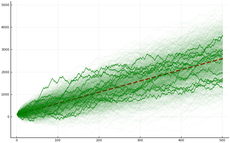
A total of 1000 simulations are run and their trajectories shown. 12 of the trajectories are randomly selected and emphasized. The red dashed curve is the predicted growth rate of $5N$ dollars profit.
Proportional Payout Gambles
Suppose I offer you a gamble: you invest 100 dollars at the start of the game; you can only withdraw your money when the game ends (you can decide when). At each round I toss a fair coin. Heads I pay into your "account" 40% of your current holdings. Tails I deduct from your account 30% of its current value.
Question 1: Should you play?
Question 2: If you do play, and say you play for $N$ rounds, how much money will you have made?
Again this looks like a winning proposition for you: starting with 100 dollars, after the toss you have 50% chance of earning 40 dollars, and 50% chance of losing 30 dollars. On the balance you come out ahead by 5 dollars (or 5% of your investment). In the long run you expect then that for each round you gain, on average, 5%; in other words your wealth multiplies by a factor of 105%. Since you are not allowed to withdraw, the earnings compound, and so you expect that after $N$ rounds, the value in your account is $ 100 \times (1.05)^N$.
Let's check this against a simulation.
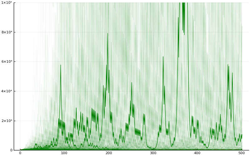
Again, a total of 1000 simulations, with 12 trajectories emphasized.
What's going on? Well, because of the exponential growth, we expect that the maximum possible pay-off is much, much larger than in the case of the fixed payout. To counteract the exponential growth and make the picture easier to see, let's plot the exact same results from the simulation but now on a semi-log plot.
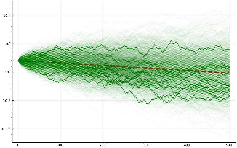
Now we put the $y$-axis on a log-scale. Still we plot 1000 simulations, with 12 trajectories emphasized. The red dashed line is not $100 \times (1.05)^N$; were it so it would have positive slope on the semi-log plot. The red dashed line is in fact $100 \times (0.98)^{N/2}$. Read on to see why.
What's going on? From the simulation it is apparent that the most-likely behavior of playing this game is that, in the long-run, your investment decreases exponentially. This is quite different from what is predicted above.
Analysis of the proportional pay-out case
Let's analyze the proportional pay-out case a bit more. First, the expectation of the payout, as computed using the $100\times (1.05)^N$ formula, is in fact correct. After playing $N$ rounds, suppose we see a total of $N_1$ heads and $N_2$ tails. Then the amount of money in the account is \[ 100 \times (1.4)^{N_1} \times (0.7)^{N_2} .\] Now, we are working with a binomial distribution, so the probability of getting $N_1$ heads and $N_2$ tails is \[ 2^{-N} \binom{N}{N_1}.\] Therefore the expected payoff, being the weighted sum of possible pay-offs by their probability, is exactly \[ E = \sum_{j = 0}^N 2^{-N} \binom{N}{j} \times 100 \times (1.4)^{j} \times (0.7)^{N-j} = \frac{100}{2^N} (1.4 + 0.7)^N = 100 \times (1.05)^N. \] What's happening, however, is that this is highly skewed by the very unlikely but super-high-earning events (say getting a vast majority of the tosses ending up heads).
This can be seen if we gather some basic statistics concerning the two settings. In the case of the fixed pay-out, our run with $N = 500$ and a total of 1000 simulations yield
Mean = 2610.185
Median = 2600.0
Max = 5400
This is exactly as expected: the possible outputs should approach a normal distribution centered at the expected mean.
Now, look at the case of the proportional payout. Our run yields
Mean = 1.06315e9
Median = 0.6405
Max = 2.81695e12
Notice how that the median is tiny while the mean is huge, indicating that we have a skewed distribution.
So what's up with the decaying overall pay-out? To understand this, notice that the most likely outcome for tossing a fair coin $N$ times, is getting about $N/2$ each of heads and tails. In this case, the amount in the account after the game ends is \[ 100 \times (1.4)^{N/2} \times (0.7)^{N/2} = 100 \times (0.98)^{N/2}. \] This explains what we saw in Figure 3, as well as the median computation.
Lessons?
The mathematical notion of an expectation value may fail to agree with what is an intuitive notion. In particular, the mathematical notion of an expectation value, taking a frequentist interpretation, is the mean over all possible outcomes (assuming equal probability of each outcome). However, one can argue that the intuitive notion of an expected outcome is the outcome corresponding to the most likely event. In the case of our game, we can argue that taking the various different head-tail tallies, the mode (which corresponds to equal numbers of each) represent the most likely event. And the outcome corresponding to the mode can, therefore, arguably be the expected outcome.
This is not a problem in many typical settings where the underlying probability distribution is normal. In fact, if we have a distribution where the mean and the mode and the median all agree, then this distinction will not show up. However, as we saw, in the proportional pay-out setting the distribution is heavily skewed, and this difference becomes significant.
The mathematical notion of an expectation value assumes it makes sense to put a linear structure on the codomain of the function. However, the linear structure on the codomain may or maynot be unique (or appropriate). In notation: let $(\Omega, \Sigma, \mathcal{P})$ be a probability space, and let $X:\Omega \to \mathbb{R}$ be a random variable. Let $f:\mathbb{R}\to \mathbb{R}$ be a measurable mapping. Then in general $f(E[X])$ and $E[f(X)]$ have absolutely nothing to do with each other! When $f$ is a bijection you can certainly argue that $X$ and $f(X)$ should have similar statistics, in terms of what is "most likely".
In the case of the proportional pay-out game, since we expect some sort of exponential growth, one can argue that it makes less sense to consider the expectation value of the payout, and more sense to consider the "expected rate of growth". (One particular justification is this: for the fixed payout game, the amount of profit is essentially independent of the starting amount you have. For the proportional payout game, the amount of profit is proportional to how much you invest originally. This shows that in the first case we have a natural additive structure, and in the second a multiplicative structure.)
One can compute the rate of growth of one trajectory by taking the amount $X_N$ at the end of game, divide it by $X_0$ the initial amount, and computing the growth rate via \[ \text{rate} = \frac{1}{N} \ln \frac{X_N}{X_0} \] If we take the mean of the growth rate as such, we will find the rate to be equal to $\ln(0.98)$.
The difference between the mean and the mode/median seen above also has the following interpretation: the behavior of the mean is what the house (taking the gambling analogy) should care about; the behavior of the mode is what the casual players usually care about.